Stats Cheatsheet!

Tests

Parametric

GLM
T-test
T-tests are handy to do and produce easily understandable results. However, they shouldn't be used for multiple comparisons as it often gives you type 1 errors (false positives). Bonferroni correction/using p-adj values can help avoid type 1 errors!
Pearson's Correlation
ANOVA/ANCOVA
Linear Regression

Non-Parametric

Wilcoxon (equivalent to 1-sample t-test)
Mann-Whitney (equivalent to 2-sample t-test
Wilcoxon matched pairs (equivalent to paired t-test
Kruskal-Wallis
Spearman's Correlation (equivalent to Pearson's correlation)
Chi-Squared

Hypergeometric (Fischer's Exact)

An association test between 2 groups. Basically a GSA algorithm but with no functional annotation via a reference genome. It'll output a p-value indicating whether two groups have more significant genes in common than expected, i.e., they are more associated than expected.To perform this test in R, you should merge the two datasets of differentially expressed genes you want to compare, get the size of the sets of significant genes for each group as well as the overlap between these numbers, and then obtain the differences. After you've done this you can perform the actual test. Here's the generic R code of all this:


        # merging tables (de = differentially expressed genes)
        de_merged = merge(de_1, de_2, by=0)
        names(de_merged) = c("log2fold_1","p_1","padj_1", "log2fold_2","p_2","padj_2")
        
        # calculate the set and overlap sizes of the groups:
        group1 = nrow(subset(de_merged, padj_1 < 0.05))
        group2 = nrow(subset(de_merged, padj_2 < 0.05))
        overlap = nrow(subset(de_merged, padj_1 < 0.05 & padj_2 < 0.05))

        # calculate the differences:
        group1_dif = group1 - overlap
        group2_dif = group2 - overlap
        total = nrow(de_merged)
        
        # the actual test:
        phyper(Overlap-1, group2, Total-group2, group1,lower.tail= FALSE)

Tukey test

Parametric tests allow you to make predictions from your model (make estimates from coefficient parameters). However, they rely on assumptions not being broken to produce reliable predicted values. The term GLM encompasses a wide range of parametric tests: t-test, ANOVA etc are different methods of fitting linear equations to data in order to model and predict. Click here to see a diagram explaining this! (opens in a new tab)

Non-parametric tests do not rely on assumptions and can handle things like outliers and non-gaussian distributions as they rank the data. However, due to this ranking, you can't make predictions using them, so they are less powerful than parametric tests.

Probability Density Functions

PDFs describe probability distributions, which are determined by the type and spread of data you're sampling from. The PDF will influence the likelihood of observing a particular value.

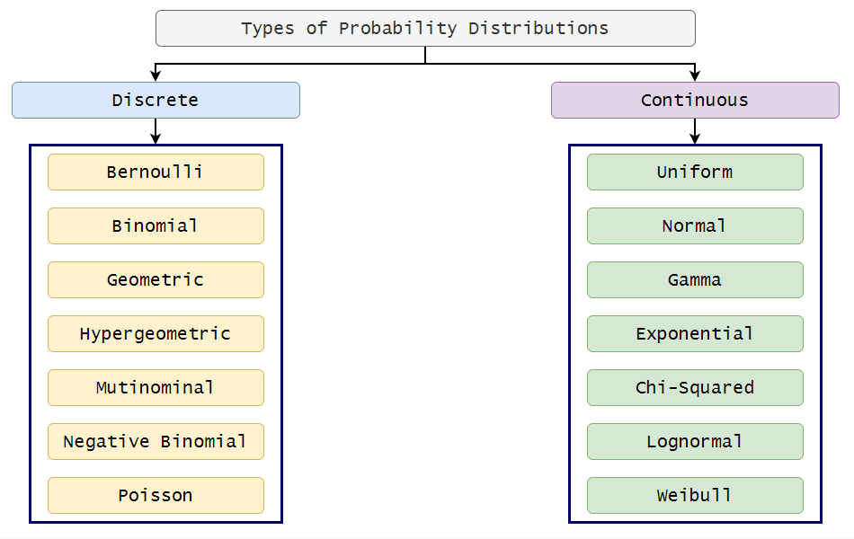
Discrete distributions have bounded values, for example binomial distributions can only take binary values, and poisson distributions can only take positive integers. This means that the outcome/predicted values from these distributions are bounded, i.e., there is a finite range of possible predicted values. Conversely, continuous distributions can take any value, up to infnite values, which translates into an infinite/unbounded range of predicted values.

Distributions are defined by their own parameters. For example, the normal distribution is defined by a mean and standard deviation.

Discrete distributions have link functions when you're trying to fit them to a linear model. The purpose of the link function (lambda or log for poisson and logit for bernoulli) is to link the outcome variable (which, if sampling from a discrete distribution, must be bounded) to the continous, unbounded linear model method. Essentially it prevents you from having silly predicted values. For example in an experiment on survival where the distribution is bernoulli and the values are either Survived(1) or Died(0), the logit link prevents the model from calculating outcomes better than 1 or worse than 0.

For reference, here's what the distributions look like modelled on histograms:

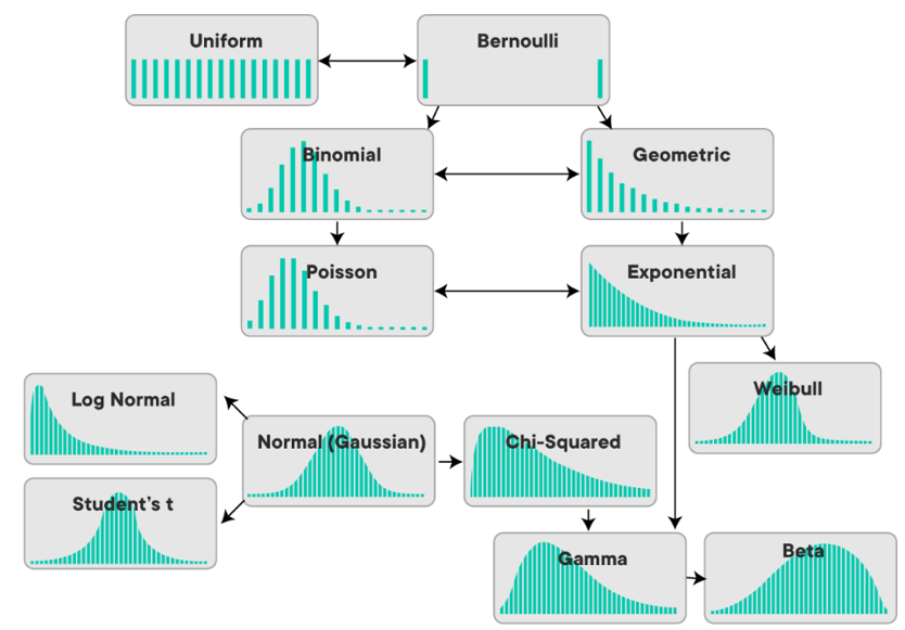
There's a lot of maths going on under the hood of PDFs. Click here for a kind of wonderful but a bit scary infographic of PDFs and the mathmatical relationships between them, taken from this paper and made into a poster by this person on reddit.

GLM Assumptions

The 4 Checks and how to check em:

Are your residuals approximately normally distributed?
If residuals are abnormally distributed, it means there is unaccounted for structure in your data that should be represented (e.g., by addition of further explanatory variables to the model). Standard error estimates for coefficients are affected when this assumption is broken.
Distribution of residuals can be checked by plotting a histogram of them and eyeballing it. The Shapiro-Wilk normality test can also be used. It tests the null hypothesis that the residuals are normally distributed. However, if your sample size is either very large or very small, you can't really trust the p value output by the test. More data gives you more power to detect small deviations from normal distribution, and the SW method tends to exaggerate the significane of these small deviations. Conversely, it will minimise deviations in a small sample size.

R code for Shapiro-Wilk: shapiro.test(my_data$myvariable)

R code for plotting distribution of residuals:
```
# make object containing residuals of model:
         res1 = resid(model1)
         # plot normality:
         qqnorm(res1) 
         
```
Are your residuals independent of each other?
I.e., is there a pattern to your residuals? If knowing something about 1 residual data point allows you to infer anything about the next one, your residuals aren't independent and you are overestimating your residual degrees of freedom and thus the power of your model! Thou shalt not pseudo-replicate. Pseudo-replication (treating variables which depend on one another as independent) will lead to more Type 1 errors. You can check for independence of residuals by plotting a scatter graph and seeing if there is any patterns or clustering of the residuals data points. Ideally, you should know in advance if your residuals aren't independent, it should be fairly obvious from the data youa re working with.
R code for testing independence of residuals:
```
# make object containing residuals of model:
         res1 = resid(model1)
         # plot scatter graph:
         scatter.smooth(res1) 
         
```
Is the variation in the response variable constant with respect to the explanatory variables? (Homogeneity/homoscedacity of variance)
If not, (a state which is called heteroscedascity), it could mean that there is unnacounted-for structure in your data. A scatter plot of the relationship between response and each explanatory variable should let you judge this. If there is heteroscedacity, the overall shape of the graph will be a fan shape, or otherwise odd-looking. There should be a smooth and constant trend in the data points.
Have you correctly interpreted any collinearity in your explanatory variables?
Not strictly an assumption but important to consider in biology. Co-linearity is strong correlations between explanatory variables. For example, if one explanatory variable is the right hand and another is the left hand. This is another one that'll be fairly easy to spot before you even get to the statistical analysis stage, however, you can also get an account of it by calculating either the sequential sums of squares or the adjusted sums of squares of the model. For example, the right hand sums of squares is 6000, but the right hand variation when the left hand variation is accounted for (i.e., the sequential/adjusted sums of squares value) is only 66. If not accounted for, co-linearity can influence parameters and standard error. The standard error being messed up means your p and T values could also be messed up, ultimately making your model outputs unreliable.

Calculations

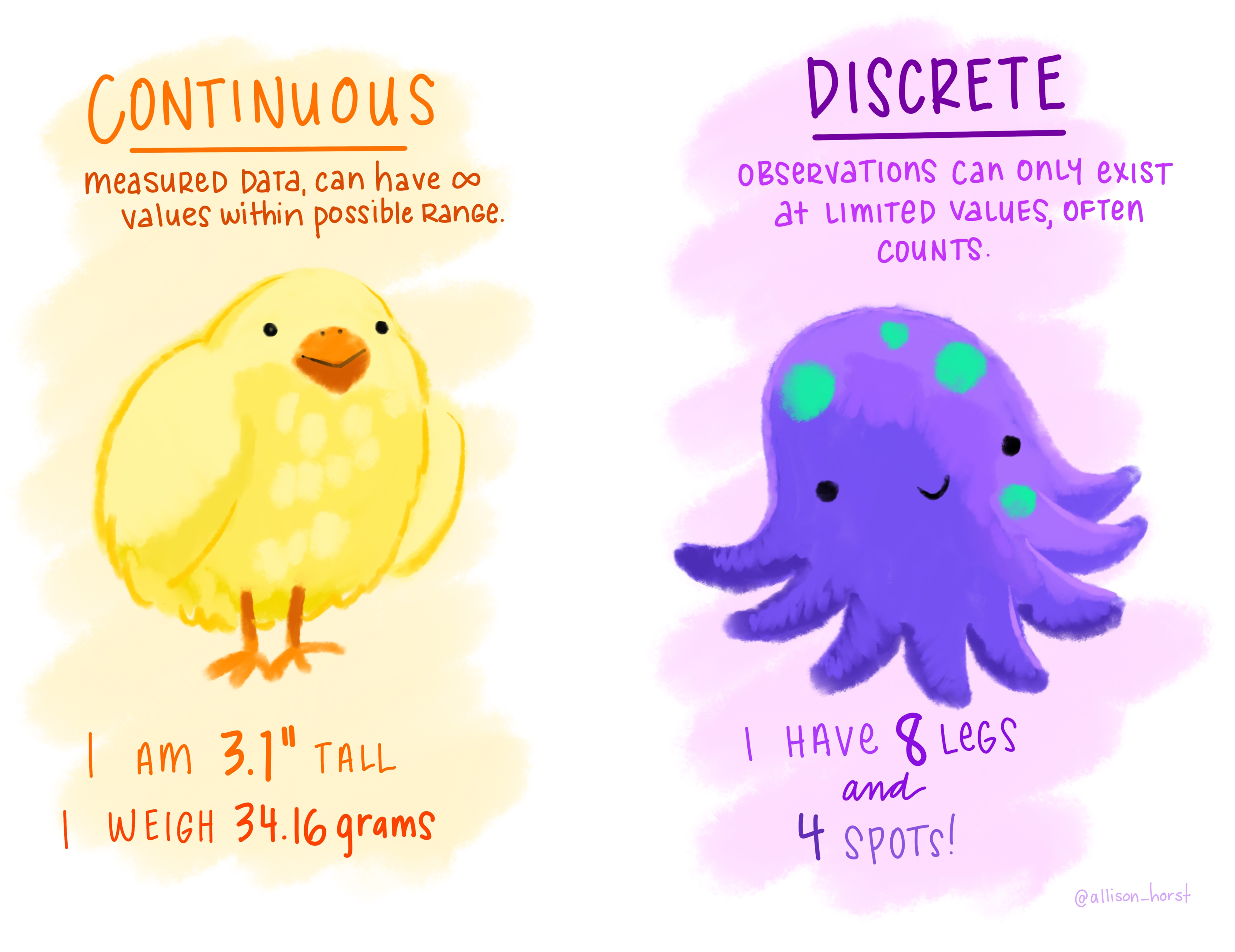
R squared = 1- RSS/TSS

Types of variables

Artwork by Allison Horst (@allison__horst)

What do to if GLM assumptions are broken

Transformation
Basic Data transformations:
- Square root
- Inverse transform (y = -1/y)
- Box-Cox
- Log2 or log10: For multiplicative change
- Z-score: For change relative to baseline
- Logit log(p/(1-p)): To linearise proportions
Generalised Linear Model or Linear Mixed Effects Regression
Non-parametric tests

Common Interpretation Pitfalls

R Snippets

Extra

The role of a model is to identify and account for all the dependencies between the data points, leaving only independent variation amongst the residuals

Measures of centrality:

Mean
Median
Mode

Measures of variation:

Range
Interquartile Range
Sums of Squares
Variance
Standard Deviation